Optimising Cab Routes In NYC Using Data

These days, on my cab rides, I have met some interesting folks driving the cabs. And, a lot of those times, when the driver was owner of the cab, our conversation tended towards to the ever-so-important question - “How to generate maximum revenue?”

Do I drive at night? Where do I start my trip? What do I optimize for – longer rides in a longer time or repeated shorter rides in the same time? How long do I drive? and alike questions. There’s a lot of other factors as well, apart from just money that can motivate a cab driver’s decisions - for the purpose of this study those are not addressed.

So, the idea was to design something very basic which could answer these questions and see the degree to which the algorithm would help the cab driver optimise, over and beyond his current earnings. I had some access to cab data released by NYC Taxi & Limousine Commission from NYC for April ‘13 capturing drop-off and pick-up co-ordinates and time of the day for all cab drivers, along with the total fare split (fare + tips). Similar data for different time-period is available on Kaggle in case any of the readers are interested to undertake the exercise on their own. The entire script is available on here.

Interesting Insights

As a part of data exploration, I tried to dig into the data to get some insights. Here are some of the interesting insights that I could gather, rest of them are plotted in the notebook.

Insight 1 - Busiest times of the day

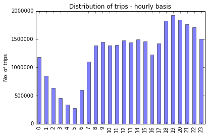It starts to drop off sharply at 12 in the night, picks up in the day around morning 8, slackens a bit towards late afternoon, and then peaks at 7 in the night.

Insight 2 - Busiest locations in the city

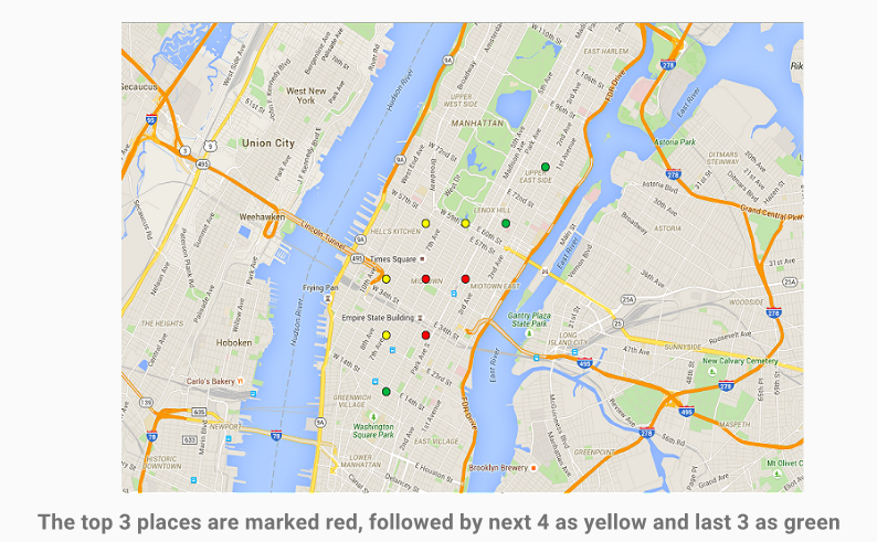
The busiest location in the city happens to be an area of 1 sq km around Park Avenue in Manhattan, NYC ( I’ve never been to NYC, just guessing from top 10 busiest locations in NYC, Manhattan seems to be the most happening place !)

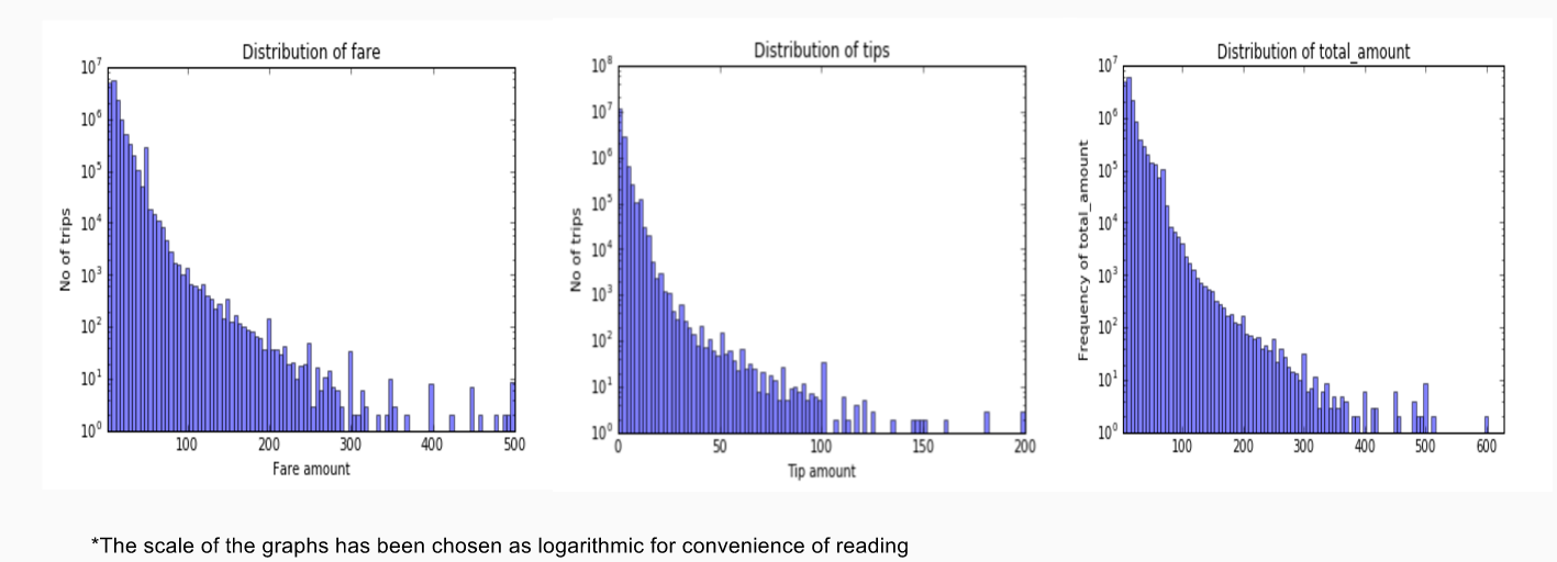
Insight 3 - Non-Gaussian fare & tips distribution

Regarding the fare distribution, I was expecting a Gaussian distribution but to my surprise it turned out to be a Poisson. The other more interesting insight was that that in tips the median was roughly 25% of the fare amount. Also, look at the outlier in the tip amount, it goes as high as $200 (that makes suddenly the driving business so lucrative !)

Insight 4 - Monday blues !

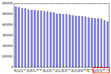Interestingly , looking at the patterns of trips for each day of the month, it’s clearly evident that Mondays of the month (1,8,15,22,29) are days with least no of trips . Though 1st was just after Easter Weekend, so presumably the least no. of trips that days justifies for itself.

Going into optimization problem

The first problem was the data was too huge for me to work on my laptop in a small time-frame. So with loss of generality, I cut down on the size by choosing the least, sampling just a single day’s data for purpose of optimizing the revenue of cab-driver.

Though the algo can very well be generalized to any number of day’s data if required. There were a few basic assumptions that I had to carve out for myself for estimating the revenue generation.

The Assumptions

• The grid chosen above would be fairly good representation of the dynamics of NYC  and that’s because 1 lat ~ 112 km and 1 long ~ 90 km (at 40 degree lat), so the chosen grid ~600sq km contains >90% of the overall rides
• For optimization of earnings, I have optimized fare amount earnt and not total amount
• There’s a linear relationship between trip fare and trip time, which is to a good extent true, as I could fit a linear regression curve with linear, square & cubic coefficients for time(in minutes) and the coefficients were orders of magnitude separate, proving it’s a linear relationship. (Appendix 2 in the Notebook)
• It’s assumed a driver can choose his own route i.e. find a customer always depending on the route he chooses
• The demand, fare, and trip time for any route and any pickup region don’t vary much within an hour and central measure is a good approximations
• Given there was no information on supply of cabs at a location, it was assumed to be proportional to demand. Hence the probability of getting a cab was assumed uniform, only the demand was checked for a threshold (higher than 20% of the median demand across all regions)
  

The Equations

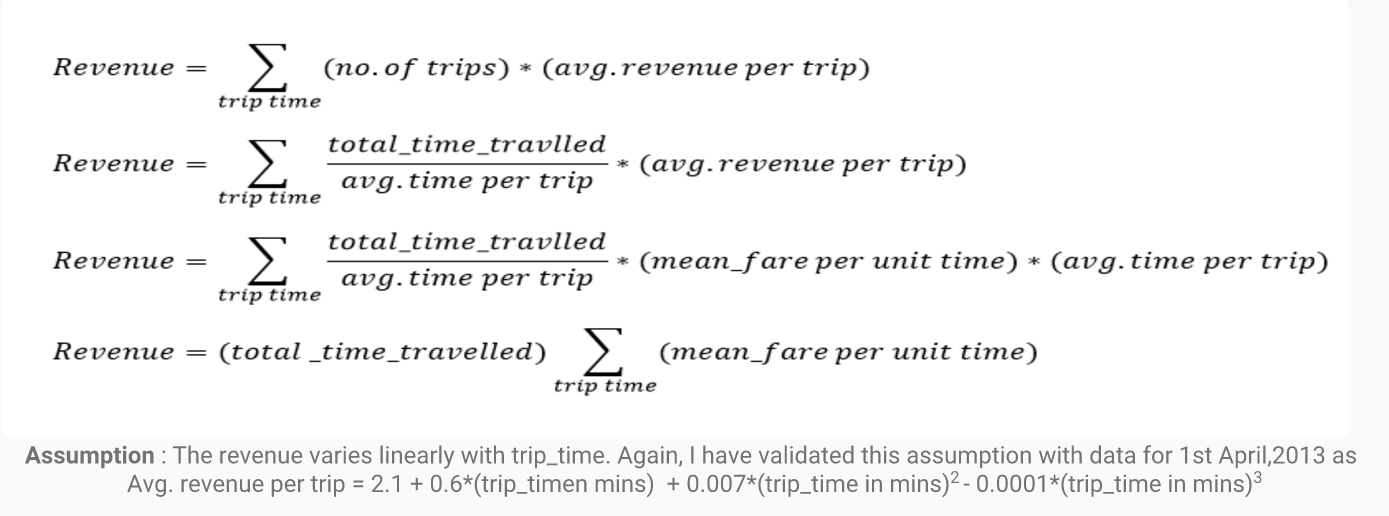
In the above equation point to be noted is the

total_time_travelled = trip time - stationary_minutes

For going from Step 2 to Step 3, the assumption (mentioned in the footer and proved in Appendix) would work fine. So from the above equations it is clear that for a cab driver to optimize his earning, he would need to optimize for 2 parameters given he has a fixed trip time

1. Mean fare per min - The cab should ideally operate on routes that have the maximum fare per min at that hour
2. Trip_time - That is, the cab should never stop in the entire duration. Ideally it should be traveling into demand regions with a minimum demand

Thus to take care of the point 2, check for the last assumption - only places with demand greater than 20% (a heuristics based threshold) median demand were considered as possible candidate locations for next trip in the optimization algorithm. If we have supply information, this could be modeled even better. Rest of the optimization algorithm boils down to maximizing point 1, i.e. Mean fare per min.

The pseudo algorithm would go something like this

1. If starting the day, then search for the region with highest mean fare per min and drive till there before you start the day
2. If drive needs to go to next day, beyond 23:59, make necessary adjustments
3. For selecting the itinerary apply recursively the function to select next best route if end_time is not crossed is as follows
   • For selecting next route,
   1. List all the  drop-off locations for which people have used cabs at the start_locaton at the start_time
   2. Calculate  the time taken to travel to each of the locations
   3. Check for the demand at each of the locations and check if they are above the threshold (20% of median of threshold)
   4. Check for the best mean_fare per min across all the routes and choose the best
   5. Calculate the time of travel & estimated fare based on data
   6. After reaching the dropoff location,adding a 3 mins for transaction, next route selection algo is applied again   - If there’s no demand for any cab at the current location (normally happens around late_night) or demand below threshold at all possible dropoff locations
   7. Do a 1 degree search for the nearest square on grid which has demand
   8. For multiple regions with demand, choose the region with best “mean fare per min” route starting from that region
   9. Estimate the time of travel to the region chosen above and add no fare to the corresponding journey
   10. If no region found having demand in 1-degree search, keep on increasing degree of search till the best location is found

Time For Results

So, now checking for the efficiency of optimisation algorithm, the benchmark is - a normal cab driver earns trip_fare of $177 (median) in roughly 6 hours (median)

Insight 5 - Hardworking and rich driver

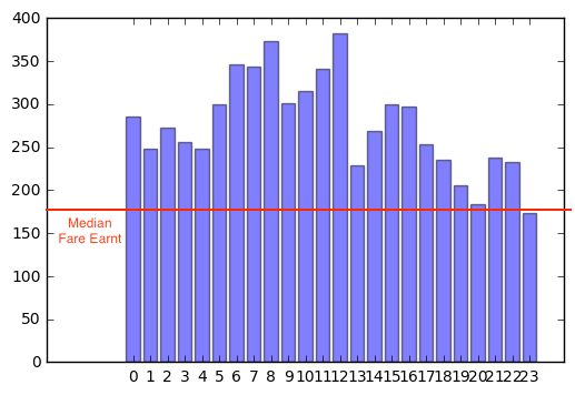The graph above shows are the fares a cab driver could earn starting out at different hours in the day using the optimisation algorithm described above (assuming he works for the median duration 6 hours).The red line marks the median fare of $177 earnt by most of the cab drivers. As is evident, the optimisation algorithm would help in earning almost every time in earning way more than the median amount.

And as it turns out if he starts at 12 noon and continues till 6 in the evening, he would earn $380 using the optimisation algorithm, which is 2.16 times more than the median fare earned by a cab driver in NYC, working for 6 hours.

Insight 6 - Efficient but lazy driver

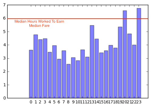The graph above depicts the time taken by a cab driver to earn the median fare of $177 using the optimisation algorithm described above, starting at different hours of the day. The red line marks the median time of 6 hours taken by most of the cab drivers.As is evident here also, the optimisation algorithm would minimise the time almost every time to way below 6 hours.

For a driver who is lazy and just wants to earn the median fare amount ($177) in quickest possible time, it turns out, if the driver starts at 8AM, he can earn the $207 in just 2 hrs 33 mins, compared to 6 hours for majority of the rest of the drivers

Conclusions

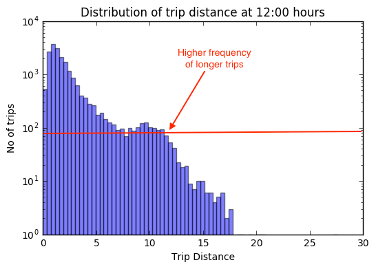
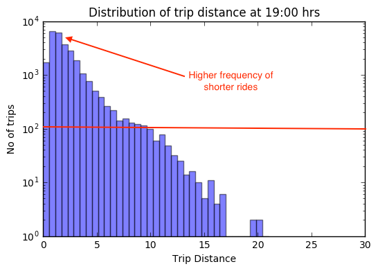
As is evident, from the above cases, the optimisation algorithm performs quite good. Though something that baffled me was why despite peaking of traffic in the evening from 18:00 -22:00 (see the busiest hours plot in the start) , it seems that as a cab driver you’re not going to make much of money starting say around 19 and driving for 6 hours as compared to starting at 12:00 hours. Also, if you’re a lazy driver, you’re going to take a lot more time to make $177 than starting at 12:00 hours.

The reason lay evident on digging a bit more into the data. Looking at the trip_distance distribution at these 2 times, it’s clear that the extra traffic peak at 19:00 hours, seems to be coming from a lot of short distance trips. In fact, frequency of trips with 10km or higher is lower at 19:00 hours.